How do you take into account correlation in error propagation?

In the error propagation formula I wrote down, we assume there are no correlated systematic uncertainties. An example of a correlated systematic would be for the case of a ruler that has some error. A ruler will measure lengths with some fractional error of $\Delta L/L$, but if its ticks are a little too long, or too short, then its measurements of the height and width of a rectangle will both be a little too short, or both too long. The amounts the values differ from the ``true'' values will be correlated. You will have to take into account the correlation of the measurements when you estimate the uncertainty on the area. If you calculate area from the product of height and width, your answer will be more likely to be too small or too large than if you used different, randomly-off ruler errors for height and width. Quantitatively, the correlation is taken into account in error propagation using a quantity called covariance, often denoted $\sigma_{xy}$.

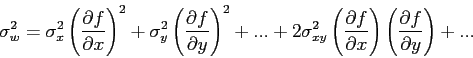
Here is the more general error propagation formula:

For some quantity $w=f(x,y,...)$, the variance of $w$, $\sigma_w^2$ (what we've been calling $(\Delta w)^2$), is given (to first order) by

$$\sigma_w^2 = \sigma_x^2 \left(\frac{\partial f}{\partial x}\r... ...tial x}\right)\left(\frac{\partial f}{\partial y}\right) + ...$$

More generally, any two variables can be correlated, like heights and weights of people in a population, and one can describe the spreads of the distributions with variances and covariances. (There's also such a thing as anti-correlation, when a large value of one variable means that the value of the other variable is more likely to be small.)

But this is a whole subject in itself. This stuff comes up a lot all over science and engineering, and you will probably bump into it if you haven't already. In this class we will pretty much assume uncorrelated uncertainties (independent variables) though.