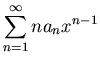
Instructor: Robert G. Brown Room 206
Texts: Arfken, Jackson (and Wyld, optional). Phone: 660-2567
Course Description In this course we will cover the following basic topics:
There will be, as you may have guessed, lots of problems. Actually, there won't as many as last year, but they'll seem like a lot as they'll be considerably harder. The structure and organization of the course will be (approximately!):
The way my grading scheme typically works is that if you get below a 50 and have not religiously done (well!) and handed in your homework, you fail (U). If you get less than a 60 and have not religiously handed in your homework, you get an (S). If you get 60 or more you get a G or E of some sort and ``pass''. If you have religiously done your homework, but have somehow managed to end up less than a 60 or (worse) 50 you may make sorrowful and wounded noises and perhaps get a G- or S, respectively. If you have not done and handed in your homework on time or have not followed the rules with respect to your homework, don't bother me about your grade - it will likely be bad and you will deserve it. Note that if you get as little as 80 per cent of your homework credit, you will only need 40 percent of your exam credit to get at least a G-.
The RULES are very serious. In previous years, certain students have reportedly betrayed the trust inherent in the rules. This has led to calls that the rules for this course (and all graduate courses here) be stringently tightened. I would prefer NOT to see this happen, as I think that the rules optimize the learning process as the stand and minimize Mickey Mouse interactions as well, but IF I get any hint of misbehavior (verified or not) I'll tighten things up very, very quickly and we'll all have to work harder and be more frustrated while working. So, PLEASE! Follow the spirit as well as the letter of the rules. You are here to learn your chosen profession, and it has never been truer that choosing an easy path is ultimately cheating yourself. Besides, it will show up on prelims!
Rules:
Research Project: I'm offering you instead the following assignment, with several choices. You may prepare any of:
If you choose to do a project, it is due TWO WEEKS before the last class2 so don't blow them off until the end. It is strongly recommended that you clear the topic with me, too.
I will grade you on: doing a decent job (good algebra), picking an interesting topic (somewhat subjective, but I can't help it and that's why I want to talk to you about it ahead of time), adequate preparation (enough algebra), adequate documentation (where did you find the algebra), organization, and Visual Aids (pictures or interactive demos are sometimes worth a thousand equations). Those of you who do numerical calculations (applying the algebra) must also write it up and (ideally) submit some nifty graphics, if possible.
I'm not going to grade you particularly brutally on this -- it is supposed to be fun as well as educational. However, if you do a miserable job on the project, it doesn't count. If you do a decent job (evidence of more than 20 hours of work) you get your ten percent of your total grade (which works out to maybe a third-of-a-grade credit and may be promoted from, say, a G+ to a E-).
I will usually be available for questions after class. It is best to make appointments to see me via e-mail. My third department job is managing the computer network (teaching this is my second and doing research is my first) so I'm usually on the computer and always insanely busy. However, I will nearly always try to answer questions if/when you catch me. That doesn't mean that I will know the answers, of course ...
Our grader is Matt Sexton, Room 203A, 660-2566, and is also generally available for help in the coursework. He has tentatively set ``office hours'' at 2:30 to 3:30 Tuesday afternoons (plus runover allowance). He will answer questions too, when He can. Otherwise He'll look busy and say that He needs to think about it and come bug me. I, in turn, will look puzzled and say I'll think about it and spend all night in the library trying to figure it out so I can tell her and she can tell you. I find (e.g.) Jackson problems just as hard as you do -- and I've done a bunch of them a bunch of times.
I welcome feedback and suggestions at any time during the year. I would prefer to hear constructive suggestions early so that I have time to implement them this semester.
I will TRY to put a complete set of lecture notes, printed out like this up on the Web in both PS and html/gif form. Exemplary problems from other sources may also be included.
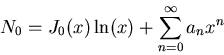
| (1) |
If we divide out the
![]() , this
becomes:
, this
becomes:
| (2) |
Fuch's Theorem
 |
(3) |
Example: Bessel (Differential) Equation
| (4) |
| (5) |
...follows directly from Fuch's Theorem:
| (6) |
 |
(7) | ||
 |
 |
(8) | |
 |
 |
(9) |
 |
(10) |
Examine the coefficients of:
 |
(11) |
We can now reconstruct the entire solution:
 |
(12) |
Remarks:
| (13) |
![]() is ordinary.
is ordinary. ![]() are regular singular points. Start
with
are regular singular points. Start
with ![]() . Using same expansions for
. Using same expansions for ![]() as above:
as above:
 |
(14) |
With a little work (and treating the first two carefully) we find that
 |
|||
 |
(15) |
 |
(16) | ||
 |
Remarks:
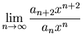
The solution is supposed to exist on the interval ![]() (right up
to the nearest singular points). If one examines the limit of the
ratio of two successive terms (the ratio test) one finds that:
(right up
to the nearest singular points). If one examines the limit of the
ratio of two successive terms (the ratio test) one finds that:
 |
 |
||
 |
|||
| (17) |
If ![]() is an integer, one of the two independent series
terminates, giving a finite polynomial solution that is defined at the
end points. The other (as it turns out, see e.g. - Courant and
Hilbert for discussion) diverges and must be rejected. We can tabulate
these solutions for each
is an integer, one of the two independent series
terminates, giving a finite polynomial solution that is defined at the
end points. The other (as it turns out, see e.g. - Courant and
Hilbert for discussion) diverges and must be rejected. We can tabulate
these solutions for each ![]() (including some optional normalization
so that
(including some optional normalization
so that ![]() ):
):
| (18) | |||
| (19) | |||
| (20) | |||
 |
 |
(21) | |
| (22) |
| (23) | |||
| (24) | |||
 |
(25) | ||
 |
(26) | ||
| (27) |
Another solution exists around the ![]() points with a
radius of converge of 1,
points with a
radius of converge of 1,
![]() . We'll look at this later, maybe.
. We'll look at this later, maybe.
| (28) |
![]() is a regular singular point, so we try:
is a regular singular point, so we try:
| (29) | |||
| (30) | |||
| (31) |
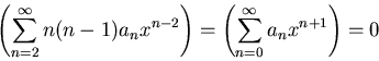
Substituting these into the ODE we obtain:
 |
(32) |
| (33) |
| (34) |
| (35) |
| (36) |
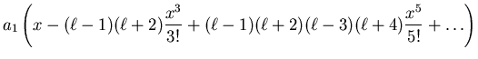
Reconstructing the series is now easy:
 |
(37) |
 |
(38) |
We will shortly solve the general case for ![]() . Or, I should
say, you will for homework. The general theory of solutions around a
regular singular point suggests that we should try a second solution
of the form:
. Or, I should
say, you will for homework. The general theory of solutions around a
regular singular point suggests that we should try a second solution
of the form:
 |
(39) |
Suppose we are given (by God, if you like) an interval ![]() , a
``weight function'' (or density function)
, a
``weight function'' (or density function) ![]() , and a set of
reasonably smooth linearly independent functions
, and a set of
reasonably smooth linearly independent functions ![]() defined on the entire interval. These functions are orthogonal
if:
defined on the entire interval. These functions are orthogonal
if:
| (40) |
| (41) |
| (42) |
| (43) |
| (44) |
We could also (if we wished) absorb ![]() into the orthogonal
representation, but it is not always useful to do so. In fact, it is
not always useful to normalize to unity - sometimes we will use an
into the orthogonal
representation, but it is not always useful to do so. In fact, it is
not always useful to normalize to unity - sometimes we will use an
![]() -dependent normalization to help us cancel or improve a factor that
appears elsewhere in our algebraic travails.
-dependent normalization to help us cancel or improve a factor that
appears elsewhere in our algebraic travails.
Note that orthogonal (or orthonormal) functions are very useful in physics! They are the basis of functional analysis, both in quantum mechanics and in the DE's of the rest of physics as well. Hence our formalization of the process:
Notation: Let
![]() ,
,
![]() ,
,
![]() , etc. Then we can notationally formalize
the relationship between functional orthogonality and the
underlying vector space with its suitably defined norm.
, etc. Then we can notationally formalize
the relationship between functional orthogonality and the
underlying vector space with its suitably defined norm.
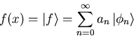
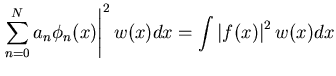
That is, suppose ![]() is a piecewise continuous function on
is a piecewise continuous function on ![]() and suppose further that the
and suppose further that the
![]() are orthogonal and
complete. Then:
are orthogonal and
complete. Then:
 |
(45) |
| (46) |
 |
|||
 |
|||
 |
(47) |
 |
(48) |
In these equations we repeatedly write down series sums over a
(possibly and indeed usually infinite) set of functions. We must,
therefore, address the issue of whether, and how, these sums converge. Noting that we were pretty slack in our requirements on
![]() - it only had to be piecewise continuous, for example, and we
said nothing about how it behaved at the points
- it only had to be piecewise continuous, for example, and we
said nothing about how it behaved at the points ![]() and
and ![]() themselves.
themselves.
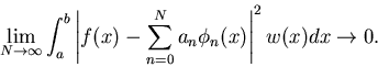
Clearly we cannot converge uniformly (at each and every point) since
at certain points the ``function'' really isn't - whether or not you
like to think that it has two values at the discontinuities, it
clearly approaches different values from the two sides in a limiting
sense that makes its value at the limit point hard to uniquely
define. It turns out that the kind of convergence that we can expect
is at least:
 |
(49) |
Note the
![]() (Cauchy criterion for convergence) inherent
in this statement. This must exist for us to be able to talk
about the sum with a straight face instead of a smirk. This is
because in the real world we cannot do infinite sums. If we make a
finite approximation:
(Cauchy criterion for convergence) inherent
in this statement. This must exist for us to be able to talk
about the sum with a straight face instead of a smirk. This is
because in the real world we cannot do infinite sums. If we make a
finite approximation:
 |
(50) |
| (51) |
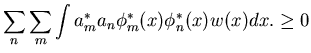
In the meantime, we can understand the fundamental idea by multiplying
out the convergence relation and noting that (since ![]() ):
):
 |
 |
||
 |
|||
 |
(52) |
| (53) |
| (54) |
Let us examine all this in the context of a well-known example.
Consider a Fourier Series for ![]() on the interval
on the interval
![]() :
:
 |
(55) |
 |
(56) | ||
 |
(57) |
With these definitions,
 |
(58) | ||
 |
(59) | ||
 |
![$\displaystyle \left[ \frac{a_0^2}{2} +
\sum_{n = 1}^{\infty}\left(\left\vert a_n \right\vert^2 + \left\vert b_n \right\vert^2 \right) \right] \pi$](img158.png) |
(60) |
If we use only the ![]() functions, they are orthogonal but not
(by themselves) complete. The expansion may only poorly approximate
the function and
functions, they are orthogonal but not
(by themselves) complete. The expansion may only poorly approximate
the function and
 |
(61) |
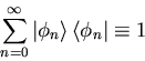
Now we can state the closure relation that is directly and
intimately connected to completeness. Assume that an orthonormal set
has ![]() (or that we have absorbed the weight factor into the
normalized functions). Then:
(or that we have absorbed the weight factor into the
normalized functions). Then:
 |
(62) | ||
 |
|||
 |
(63) |
But:
| (64) |
 |
(65) | ||
 |
(66) |
| (67) |
To continue using Fourier representations as an example, consider the
normalized function:
| (68) |
 |
 |
(69) | |
| (70) |
In many cases one can obtain a linearly independent set of functions
![]() , but find upon examination that they are (alas!) not
orthogonal. For example,
, but find upon examination that they are (alas!) not
orthogonal. For example, ![]() . Fortunately, it is always
possible to orthogonalize the set of functions via a simple
procedure. Let us define
. Fortunately, it is always
possible to orthogonalize the set of functions via a simple
procedure. Let us define ![]() to be the set of non-orthogonal
but linearly independent functions. We will take suitable linear
combinations of them to generate an orthogonal set which we will call
to be the set of non-orthogonal
but linearly independent functions. We will take suitable linear
combinations of them to generate an orthogonal set which we will call
![]() . Finally, we can normalize this orthogonal set any
way we like to form a orthonormal representation
. Finally, we can normalize this orthogonal set any
way we like to form a orthonormal representation ![]() .
.
To understand the Gram-Schmidt procedure, it is easiest to consider it
for ordinary Cartesian vectors. Suppose ![]() and
and ![]() are
two non-orthogonal, but linearly independent vectors that span a
two-dimensional plane as drawn below:
are
two non-orthogonal, but linearly independent vectors that span a
two-dimensional plane as drawn below:
In this figure, we see that we can systematically construct
![]() by projecting
by projecting ![]() onto
onto ![]() and subtracting
its
and subtracting
its ![]() -directed component from
-directed component from ![]() itself. What is left
is necessarily orthogonal to
itself. What is left
is necessarily orthogonal to ![]() . Algebraically:
. Algebraically:
| (71) |
| (72) |
| (73) |
 |
(74) |
 |
(75) |
This procedure works just as well for ![]() sequential operations and
with functional ``vectors'' instead of real space vectors. Pick any
function
sequential operations and
with functional ``vectors'' instead of real space vectors. Pick any
function ![]() . Let
. Let
| (76) |
 |
(77) |
| (78) |
| (79) |
| (80) |
We then try to make
| (81) |
| (82) | |||
| (83) |
There is a clever example in both Arfken and Wyld where they show that
if you take ![]() and apply this procedure on the interval
and apply this procedure on the interval
![]() with
with ![]() , you obtain the (gasp!) Legendre
Polynomials! In fact, if one varies the interval and the weight
function, one can obtain all the known orthogonal polynomials in
this manner!
, you obtain the (gasp!) Legendre
Polynomials! In fact, if one varies the interval and the weight
function, one can obtain all the known orthogonal polynomials in
this manner!
These are quite useful for both expansions and numerical integration (quadrature).
Suppose one has a general 2nd order linear homogeneous ODE:
| (84) |
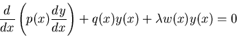 |
(85) |
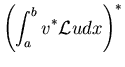
Once it is in this form, we can easily show that it has a really nifty
property. Let us define the linear operator ![]() such
that:
such
that:
![$\displaystyle \frac{d^{} }{dx^{}}\left[p(x)\frac{d^{} u}{dx^{}}\right] + q(x)u$](img212.png) |
(86) | ||
![$\displaystyle \frac{d^{} }{dx^{}}\left[p(x)\frac{d^{} v}{dx^{}}\right] + q(x)v$](img214.png) |
(87) |
![\begin{displaymath}
\int_a^b dx \left[v{\cal L}u - u{\cal L}v\right] = \left[p\l...
...ac{d^{} u}{dx^{}}
- u \frac{d^{} v}{dx^{}}\right) \right]_a^b
\end{displaymath}](img217.png) |
(88) |
| (89) | |||
| (90) |
| (91) |
| (92) |
With this observation in hand, we can easily proceed to prove 2/3 of the Sturm-Liouville Theorem for solutions to nearly general (self-adjoint) 2OLHODE's.
We assume (here as above):
Then solutions to S-L 2OLHODE are a discrete set of eigenfunctions (![]() ) and corresponding eigenvalues
(
) and corresponding eigenvalues
(![]() ) where:
) where:
Note that sometimes
![]() for distinct
for distinct ![]() 's so you
might think that the
's so you
might think that the ![]() 's don't have to be orthogonal. However, they
do have to be linearly independent or they are distinct solutions with
a vanishing Wronskian! So, we can GSO them to orthogonalize the
's don't have to be orthogonal. However, they
do have to be linearly independent or they are distinct solutions with
a vanishing Wronskian! So, we can GSO them to orthogonalize the
![]() -degenerate subspace. So for all practical purposes, after a
bit of work, all the
-degenerate subspace. So for all practical purposes, after a
bit of work, all the ![]() are orthogonal or can be made so even if
their eigenvalues are the same.
are orthogonal or can be made so even if
their eigenvalues are the same.
In summary, given a set of ![]() 's that solve a 2OLHODE, we can
always write them as a complete orthonormal set
's that solve a 2OLHODE, we can
always write them as a complete orthonormal set ![]() .
.
This is a really useful theorem. Immediately implies the
orthogonality of all the common ODE solution sets and orthogonal
function sets in use in physics, e.g.
![]() , with its
well-known Fourier solutions on the interval
, with its
well-known Fourier solutions on the interval ![]() with Dirichlet
boundary conditions
with Dirichlet
boundary conditions ![]() ,
, ![]() ,
,
![]() with
with
![]() . Whew!
. Whew!
It is easy and instructive to prove the first two properties predicted
by the SL theorem. The Hermitian property above implies:
 |
 |
(93) | |
 |
(94) |
| (95) |
| (96) |
NOW, let ![]() and
and ![]() be any two solutions
be any two solutions ![]() and
and ![]() corresponding to
corresponding to ![]() and
and ![]() . Then:
. Then:
| (97) |
| (98) |
THUS
| (99) |
| (100) |
It turns out to be quite difficult and involved to prove completeness. One basically has to show closure of one sort or another, and closure is not immediately obvious. It has long since been proven, however, and is shown in serious books like Hilbert and Courant if you want/need to look over the proof some day.
From this day forth, then, I will assume that you just know that the solutions to nearly every 2OLHODE that we treat in this course (and the rest of your courses form an orthogonal (appropriately normalized, in practice) basis, out of which it is perfectly clear that general solutions can be built via superposition.
It is time now for a short interlude, first on tensors (to get the trivia out of the way), then on curvilinear coordinates (to get you to where you can appreciate separation of variables in the Big Three coordinate systems) and we'll hop on back to ODE's, this time in the context of PDE's and ``real physics''.
| (101) |
If we divide out the
![]() , this
becomes:
, this
becomes:
| (102) |
Fuch's Theorem
| (103) |
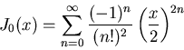
Example: Bessel (Differential) Equation
| (104) |
| (105) |
...follows directly from Fuch's Theorem:
| (106) |
| (107) | |||
|
(108) | ||
|
(109) |
 |
(110) |
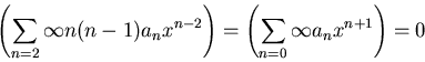
Examine the coefficients of:
|
(111) |
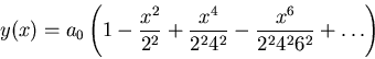
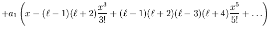
We can now reconstruct the entire solution:
|
(112) |
Remarks:
| (113) |
![]() is ordinary.
is ordinary. ![]() are regular singular points. Start
with
are regular singular points. Start
with ![]() . Using same expansions for
. Using same expansions for ![]() as above:
as above:
| (114) |
With a little work (and treating the first two carefully) we find that
|
|||
|
(115) |
|
|||
 |
(116) |
Remarks:
Iff ![]() is an integer, one of the two independent series
terminates, giving a finite polynomial solution. We can tabulate
these solutions for each
is an integer, one of the two independent series
terminates, giving a finite polynomial solution. We can tabulate
these solutions for each ![]() (including some optional normalization
so that
(including some optional normalization
so that ![]() ):
):
| (117) | |||
| (118) | |||
| (119) | |||
|
|
(120) | |
| (121) |
| (122) | |||
| (123) | |||
|
(124) | ||
|
(125) | ||
| (126) |